Deck 3: Displaying and Summarizing Quantitative Data
Full screen (f)
Question
The histogram displays the body fat percentages of 65 students taking a college health course.In addition to describing the distribution,give a reason to account for the shape of this distribution. 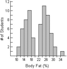
A)The distribution of body fat percentages is bimodal,with a cluster of body fat percentages around 16% and another cluster of body fat percentages around 26%.The upper cluster shows a bit of a skew to the right.Most students in the lower cluster have body fat percentages between 16% and 20%,and most students in the upper cluster have body fat percentages between 22% and 26%.Men and women have different body fat percentages: the lower cluster would likely represent male students,and the upper cluster would likely represent female students.
B)The distribution of body fat percentages is unimodal,with a bit of a skew to the right.The body fat percentages are centred around 20%,with a range of 10% to 35%.Most students have body fat percentages between 12% and 28%.Men and women have different body fat percentages,but the average of body fat percentages for men and women would be around 20%.
C)The distribution of body fat percentages is unimodal,with a bit of a skew to the right.The body fat percentages are centred around 24%,with a range of 10% to 34%.Most students have body fat percentages between 12% and 28%.Men and women have different body fat percentages,but the average of body fat percentages for men and women would be around 24%.
D)The distribution of body fat percentages is bimodal,with a cluster of body fat percentages around 16% and another cluster of body fat percentages around 26%.The upper cluster shows a bit of a skew to the right.Most students in the lower cluster have body fat percentages between 12% and 18%,and most students in the upper cluster have body fat percentages between 22% and 28%.Men and women have different body fat percentages: the lower cluster would likely represent male students,and the upper cluster would likely represent female students.
E)The distribution of body fat percentages is bimodal,with a cluster of body fat percentages around 12% and another cluster of body fat percentages around 28%.The upper cluster shows a bit of a skew to the right.Most students in the lower cluster have body fat percentages between 12% and 18%,and most students in the upper cluster have body fat percentages between 22% and 28%.Men and women have different body fat percentages: the lower cluster would likely represent male students,and the upper cluster would likely represent female students.
Question
Question
Question
Question
Question
Question
The display shows the heights of Grade 12 students at a local high school,collected so that the students could be arranged with shorter ones in front and taller ones in back for a class photograph.In addition to describing the distribution,give a reason to account for the shape of this distribution. 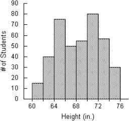
A)The distribution of the heights of Grade 12 students is bimodal,with a mode at around 65 inches and the other mode around 71 inches.The students' heights are between 60 inches and 74 inches.The two modes would likely represent the average heights of the male and female students.
B)The distribution of the heights of Grade 12 students is unimodal centred at 68,with a heights ranging from 60 inches to 76 inches.The two peaks would likely represent the average heights of the male and female students.
C)The distribution of the heights of Grade 12 students is bimodal,with a mode at around 62 inches and the other mode around 74 inches.No student has a height below 60 inches or above 76 inches.The two modes would likely represent the average heights of the male and female students.
D)The distribution of the heights of Grade 12 students is bimodal,with a mode at around 65 inches and the other mode around 71 inches.No student has a height below 60 inches or above 76 inches.The two modes would likely represent the average heights of the male and female students.
E)The distribution of the heights of Grade 12 students is uniform centred at 68,with a heights ranging from 60 inches to 76 inches.The two peaks would likely represent the average heights of the male and female students.
Question
Question
The histogram shows the lengths of hospital stays (in hours)for pregnant women admitted to hospitals in Ontario who were having contractions upon arrival. 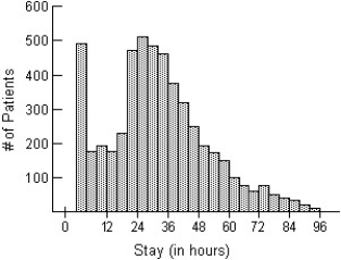
A)The distribution of the length of hospital stays for pregnant patients is skewed to the right,with stays ranging from 1 hour to 96 hours.The distribution is centred around 26 hours,with the majority of stays lasting between 1 to 48 hours.There are relatively few hospital stays longer than 72 hours.Many patients have a stay of only 1-4 hours,possibly because it was not time to deliver.
B)The distribution of the length of hospital stays for pregnant patients is skewed to the right,with stays ranging from 1 hour to 95 hours.The distribution is centred around 26 hours,with the majority of stays lasting between 1 to 48 hours.There are relatively few hospital stays longer than 72 hours.
C)The distribution of the length of hospital stays for pregnant patients is skewed to the right,with stays ranging from 1 hour to 96 hours.The distribution is centred around 26 hours,with the majority of stays lasting between 3 to 24 hours.There are relatively few hospital stays longer than 72 hours.Many patients have a stay of only 1-4 hours,possibly because it was not time to deliver.
D)The distribution of the length of hospital stays for pregnant patients is skewed to the right,with stays ranging from 1 hour to 95 hours.The distribution is centred around 48 hours,with the majority of stays lasting between 24 to 72 hours.There are relatively few hospital stays longer than 72 hours.Many patients have a stay of only 1-3 hours,possibly because it was not time to deliver.
E)The distribution of the length of hospital stays for pregnant patients is skewed to the right,with stays ranging from 1 hour to 95 hours.The distribution is centred around 26 hours,with the majority of stays lasting between 1 to 48 hours.There are relatively few hospital stays longer than 72 hours.Many patients have a stay of only 1-3 hours,possibly because it was not time to deliver.
Question
A university instructor created a website for her Chemistry course.The students in her class were encouraged to use the website as an additional resource for the course.At the end of the semester,the instructor asked each student how many times he or she visited the website and recorded the counts.Based on the histogram below,describe the distribution of website use. 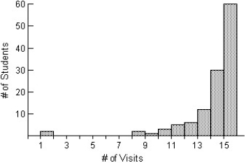
A)The distribution of the number of visits to the course website by each student for the semester is skewed to the left,with the number of visits ranging from 1 to 15 visits.The distribution is centred at about 14 visits,with many students visiting 15 times.
B)The distribution of the number of visits to the course website by each student for the semester is skewed to the left,with the number of visits ranging from 1 to 16 visits.The distribution is centred at about 14 visits,with many students visiting 15 times.There is an outlier in the distribution,two students who visited the site only once.The next highest number of visits was 8.
C)The distribution of the number of visits to the course website by each student for the semester is skewed to the right,with the number of visits ranging from 1 to 15 visits.The distribution is centred at about 14 visits,with many students visiting 15 times.There is an outlier in the distribution,two students who visited the site only once.The next highest number of visits was 8.
D)The distribution of the number of visits to the course website by each student for the semester is skewed to the left,with the number of visits ranging from 1 to 15 visits.The distribution is centred at about 14 visits,with many students visiting 15 times.There is an outlier in the distribution,two students who visited the site only once.The next highest number of visits was 8.
E)The distribution of the number of visits to the course website by each student for the semester is skewed to the left,with the number of visits ranging from 1 to 15 visits.The distribution is centred at about 12 visits,with many students visiting 15 times.There is an outlier in the distribution,two students who visited the site only once.The next highest number of visits was 8.
Question
Question
Question
Question
Question
The histogram shows the cost of living,in dollars,in 32 Canadian towns. 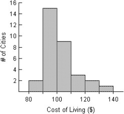
A)The distribution of the cost of living in the 32 Canadian cities is unimodal and skewed to the right.The distribution is centred around $100,and spread out,with values ranging from $80 to $139.99.
B)The distribution of the cost of living in the 32 Canadian cities is unimodal and skewed to the right.The distribution is centred around $110,and spread out,with values ranging from $80 to $140.
C)The distribution of the cost of living in the 32 Canadian cities is unimodal and skewed to the right.The distribution is centred around $90,and spread out,with values ranging from $80 to $139.99.
D)The distribution of the cost of living in the 32 Canadian cities is unimodal and skewed to the left.The distribution is centred around $100,and spread out,with values ranging from $80 to $139.99.
E)The distribution of the cost of living in the 32 Canadian cities is unimodal.The distribution is centred around $100,and spread out,with values ranging from $80 to $140.
Question
Question
Question
The histogram shows the sizes (in acres)of 169 farms in Ontario.In addition to describing the distribution,approximate the percentage of farms that are under 100 acres. 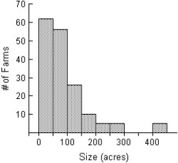
A)The distribution of the size of farms in Ontario is skewed to the right.Most of the farms are smaller than 150 acres,with some larger ones,from 150 to 300 acres.Five farms were larger than the rest,over 400 acres.The mode of the distribution is between 0 and 50 acres.It appears that 118 of 169 farms are under 100 acres,approximately 70%.
B)The distribution of the size of farms in Ontario is symmetric,with farm sizes ranging from 0 to 450 acres.The mode of the distribution is between 0 and 50 acres.It appears that 118 of 169 farms are under 100 acres,approximately 70%.
C)The distribution of the size of farms in Ontario is symmetric,with farm sizes ranging from 0 to 450 acres.The mode of the distribution is between 100 and 150 acres.It appears that 118 of 169 farms are under 100 acres,approximately 70%.
D)The distribution of the size of farms in Ontario is skewed to the right.Most of the farms are smaller than 50 acres,with some larger ones,from 150 to 300 acres.Five farms were larger than the rest,over 400 acres.The mode of the distribution is between 0 and 50 acres.It appears that 118 of 169 farms are under 100 acres,approximately 70%.
E)The distribution of the size of farms in Ontario is skewed to the right.Most of the farms are smaller than 150 acres,with some larger ones,from 150 to 300 acres.Five farms were larger than the rest,over 400 acres.The mode of the distribution is between 0 and 50 acres.It appears that 62 of 169 farms are under 100 acres,approximately 37%.
Question
Question
Question
Question
A weight-loss company used the following histogram to show the distribution of the number of pounds lost by clients during the year 2014.Comment on the display. 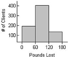
Question
The histograms display the body fat percentages of 42 female students and 48 male students taking a college health course.For which of the variables depicted in the histograms would you be most satisfied to summarize the centre with a mean? Explain. 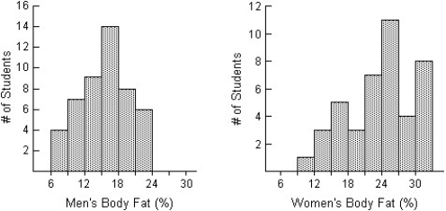
A)The histogram of Women's Body Fat is skewed on the left.That makes it the best candidate of summarizing with a mean.
B)The histogram of Women's Body Fat shows no outliers.That makes it the best candidate of summarizing with a mean.
C)The histogram of Men's Body Fat is most nearly symmetric,is not strongly skewed and shows no outliers.That makes it the best candidate of summarizing with a mean.
D)The histogram of Women's Body Fat is most nearly symmetric,is not strongly skewed and shows no outliers.That makes it the best candidate of summarizing with a mean.
E)The histogram of Men's Body Fat is skewed on the left.That makes it the best candidate of summarizing with a mean.
Question
Question
Here are summary statistics of the four last digits of social security number of 500 customers,corresponding to the following histogram.
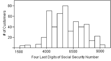 Is the mean or median a "better" summary of the centre of the distribution?
A)Neither,because these are not categorical data.
B)Neither,because these are not quantitative data.
C)Median,because the IQR is smaller than the standard deviation.
D)Mean,because the distribution is quite symmetric.
E)Median,because of the outliers.
Is the mean or median a "better" summary of the centre of the distribution?A)Neither,because these are not categorical data.
B)Neither,because these are not quantitative data.
C)Median,because the IQR is smaller than the standard deviation.
D)Mean,because the distribution is quite symmetric.
E)Median,because of the outliers.
Question
Question
Question
Question
Question
Question
In a survey,20 people were asked how many magazines they had purchased during the previous year.The results are shown below.Construct a histogram to represent the data.Use 4 bins with a bin width of 10,and begin with a lower bin limit of -0.5.What is the approximate amount at the centre?
6 15 3 36 25 18 12 18 5 30
24 7 0 22 33 24 19 4 12 9
6 15 3 36 25 18 12 18 5 30
24 7 0 22 33 24 19 4 12 9
Question
In a survey,26 voters were asked their ages.The results are shown below.Construct a histogram to represent the data (with 5 bins beginning with a lower bin limit of 19.5 and a bin width of 10).What is the approximate age at the centre?
43 56 28 63 67 66 52 48 37 51 40 60 62
66 45 21 35 49 32 53 61 53 69 31 48 59
43 56 28 63 67 66 52 48 37 51 40 60 62
66 45 21 35 49 32 53 61 53 69 31 48 59
Question
Question
Question
Question
Question
Question
Shown below are the histogram and summary statistics for the reading scores of 29 fifth graders. 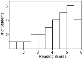 Which measures of centre and spread would you use for this distribution?
A)Mean and IQR,because the data is skewed to the left.
B)Median and standard deviation,because the data is skewed to the left.
C)Mean and standard deviation,because the data is skewed to the left.
D)Mean and standard deviation,because the data is symmetric.
E)Median and IQR,because the data is skewed to the left.
Which measures of centre and spread would you use for this distribution?A)Mean and IQR,because the data is skewed to the left.
B)Median and standard deviation,because the data is skewed to the left.
C)Mean and standard deviation,because the data is skewed to the left.
D)Mean and standard deviation,because the data is symmetric.
E)Median and IQR,because the data is skewed to the left.
Question
Students were asked to make a histogram of the number of corn snakes collected in Will County,Illinois from 1985 to 2006.They were given the data in the form of a stem-and-leaf display shown below: 
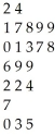

 = 57 corn snakes
One student submitted the following display: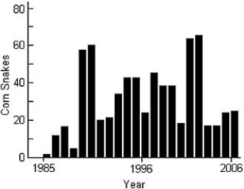 a)Comment on this graph.
b)Create your own histogram of the data.
= 57 corn snakesOne student submitted the following display:
a)Comment on this graph.b)Create your own histogram of the data.
Question
A dotplot of the number of tornadoes each year in a certain county from 1948 to 2004 is given.Each dot represents a year in which there were that many tornadoes. 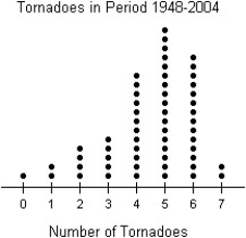
A)The distribution of the number of tornadoes per year is unimodal and symmetric,with a centre around 5 tornadoes per year.The number of tornadoes per year ranges from 0 to 7.
B)The distribution of the number of tornadoes per year is unimodal and skewed to the left,with a centre around 3.5 tornadoes per year.The number of tornadoes per year ranges from 0 to 7.
C)The distribution of the number of tornadoes per year is unimodal and symmetric,with a centre around 3.5 tornadoes per year.The number of tornadoes per year ranges from 0 to 7.
D)The distribution of the number of tornadoes per year is unimodal and skewed to the left,with a centre around 5 tornadoes per year.The number of tornadoes per year ranges from 0 to 7.
E)The distribution of the number of tornadoes per year is unimodal and skewed to the right,with a centre around 5 tornadoes per year.The number of tornadoes per year ranges from 0 to 7.
Question
Question
Question
Question
The histograms show the cost of living,in dollars,for 32 U.S.cities.The histogram on the left shows the cost of living for the 32 cities using bins $10 wide,and the histogram on the right displays the same data using bins that are $6 wide.For which of the histograms would you most strenuously insist on using an IQR rather than a standard deviation to summarize spread? Explain. 
A)The histogram on the right is most nearly symmetric and shows no outliers.That makes it the best candidate for summarizing with an IQR.
B)The histogram on the left shows a low outlier.The standard deviation is sensitive to outliers,so we'd prefer to use the IQR for this one.
C)The histogram on the right shows a high outlier.The standard deviation is sensitive to outliers,so we'd prefer to use the IQR for this one.
D)The histogram on the left is most strongly skewed to the right.That makes it the best candidate for summarizing with an IQR.
E)The histogram on the left is most nearly symmetric and shows no outliers.That makes it the best candidate for summarizing with an IQR.
Question
Question
Question
Question
Question
Question
Question
Question
Question
Question
Question
Question
Question
Question
Question
Question
The back-to-back dotplot shows the number of fatalities per year caused by tornadoes in a certain state for two periods: 1950-1974 and 1975-1999.Explain how you would summarize the centre and spread of each of the variables depicted in the dotplots. 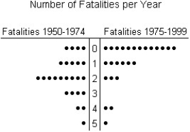
A)The distribution of the number of fatalities per year for the period 1950-1974 is unimodal and approximately symmetric.Therefore,we would be satisfied using the mean to summarize the centre and the standard deviation to summarize spread.For the period 1975-1999,the distribution of the number of fatalities per year is also unimodal,but skewed to the right.Therefore,we would prefer to use a median for centre and an IQR to summarize spread.
B)The distribution of the number of fatalities per year for the period 1950-1974 is unimodal,but skewed to the right.Therefore,we would prefer to use a median for centre and an IQR to summarize spread.For the period 1975-1999,the distribution is also unimodal and approximately symmetric.Therefore,we would be satisfied using the mean to summarize the centre and the standard deviation to summarize spread.
C)The distribution of the number of fatalities per year for the period 1950-1974 is bimodal.Therefore,we would prefer to use a median to summarize the centre and an IQR to summarize spread.For the period 1975-1999,the distribution of the number of fatalities per year is also bimodal,but skewed to the left.Therefore,we would prefer to use a mean for centre and a standard deviation to summarize spread.
D)The distribution of the number of fatalities per year for the period 1950-1974 is unimodal and approximately symmetric.Therefore,we would prefer to use the median to summarize the centre and the standard deviation to summarize spread.For the period 1975-1999,the distribution of the number of fatalities per year is also unimodal,but skewed to the right.Therefore,we would prefer to use the mean for centre and an IQR to summarize spread.
E)The distribution of the number of fatalities per year for the period 1950-1974 is unimodal but skewed to the right.Therefore,we would prefer to use a median to summarize the centre and IQR to summarize spread.For the period 1975-1999,the distribution of the number of fatalities per year is also unimodal and skewed to the right.Therefore,we would prefer to use a median for centre and an IQR to summarize spread.
Question
Question
Question
Question
Question
Question
Question
Question
Question
Question
Question
Question
Question
Question
Question
Question
Question
Question
Question
Question

Unlock Deck
Sign up to unlock the cards in this deck!
Unlock Deck
Unlock Deck
1/148
Play
Full screen (f)
Deck 3: Displaying and Summarizing Quantitative Data
1
The histogram displays the body fat percentages of 65 students taking a college health course.In addition to describing the distribution,give a reason to account for the shape of this distribution.
A)The distribution of body fat percentages is bimodal,with a cluster of body fat percentages around 16% and another cluster of body fat percentages around 26%.The upper cluster shows a bit of a skew to the right.Most students in the lower cluster have body fat percentages between 16% and 20%,and most students in the upper cluster have body fat percentages between 22% and 26%.Men and women have different body fat percentages: the lower cluster would likely represent male students,and the upper cluster would likely represent female students.
B)The distribution of body fat percentages is unimodal,with a bit of a skew to the right.The body fat percentages are centred around 20%,with a range of 10% to 35%.Most students have body fat percentages between 12% and 28%.Men and women have different body fat percentages,but the average of body fat percentages for men and women would be around 20%.
C)The distribution of body fat percentages is unimodal,with a bit of a skew to the right.The body fat percentages are centred around 24%,with a range of 10% to 34%.Most students have body fat percentages between 12% and 28%.Men and women have different body fat percentages,but the average of body fat percentages for men and women would be around 24%.
D)The distribution of body fat percentages is bimodal,with a cluster of body fat percentages around 16% and another cluster of body fat percentages around 26%.The upper cluster shows a bit of a skew to the right.Most students in the lower cluster have body fat percentages between 12% and 18%,and most students in the upper cluster have body fat percentages between 22% and 28%.Men and women have different body fat percentages: the lower cluster would likely represent male students,and the upper cluster would likely represent female students.
E)The distribution of body fat percentages is bimodal,with a cluster of body fat percentages around 12% and another cluster of body fat percentages around 28%.The upper cluster shows a bit of a skew to the right.Most students in the lower cluster have body fat percentages between 12% and 18%,and most students in the upper cluster have body fat percentages between 22% and 28%.Men and women have different body fat percentages: the lower cluster would likely represent male students,and the upper cluster would likely represent female students.
The distribution of body fat percentages is bimodal,with a cluster of body fat percentages around 16% and another cluster of body fat percentages around 26%.The upper cluster shows a bit of a skew to the right.Most students in the lower cluster have body fat percentages between 12% and 18%,and most students in the upper cluster have body fat percentages between 22% and 28%.Men and women have different body fat percentages: the lower cluster would likely represent male students,and the upper cluster would likely represent female students.
2
Heights of adult women attending a concert.
A)The distribution would likely be unimodal and symmetric.The average height of women at the concert will be about the same as the median height.The distribution will likely be symmetric,since there are some women who are taller than average and some that are shorter.
B)The distribution would likely be uniform,with the heights of women evenly distributed.
C)The distribution would likely be unimodal and slightly skewed right.The average height of women at the concert will be about the same as the median height.The distribution will likely be slightly skewed right,since there are more women who are tall than short.
D)The distribution would likely be bimodal and slightly skewed left.The average height of shorter women will be at one mode,and the average height of taller women at the other mode.The distribution will likely be slightly skewed left,since there are more women who are short than tall.
E)The distribution would likely be bimodal and slightly skewed right.The average height of shorter women will be at one mode,and the average height of taller women at the other mode.The distribution will likely be slightly skewed right,since there are more women who are tall than short.
The distribution would likely be unimodal and symmetric.The average height of women at the concert will be about the same as the median height.The distribution will likely be symmetric,since there are some women who are taller than average and some that are shorter.
3
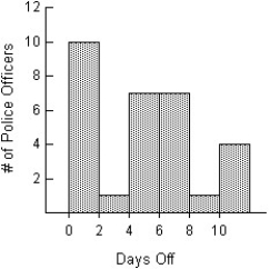
The number of days off that 30 police officers took in a given year are provided below.Create a histogram of the data using bins 2 days wide.
10 1 3 5 4 7
5 1 0 9 11 1
5 4 1 7 7 11
0 6 6 1 5 7
10 1 1 5 6 0
10 1 3 5 4 7
5 1 0 9 11 1
5 4 1 7 7 11
0 6 6 1 5 7
10 1 1 5 6 0
4
Ontario wanted to find the typical size of farms in the province.The data below shows the sizes (in acres)of the 84 farms located in Ontario.Create a histogram of the data using bins that are 50 acres wide.
200 172 52 100 85 100
50 63 16 64 40 54
8 25 212 67 125 250
400 142 65 49 45 9
32 33 41 112 99 50
88 66 135 18 37 38
103 296 98 77 85 29
73 48 48 167 15 100
149 59 80 21 141 33
21 130 49 37 139 17
95 40 5 440 21 60
19 199 147 46 90 26
61 91 28 84 47 159
182 73 71 249 50 92
200 172 52 100 85 100
50 63 16 64 40 54
8 25 212 67 125 250
400 142 65 49 45 9
32 33 41 112 99 50
88 66 135 18 37 38
103 296 98 77 85 29
73 48 48 167 15 100
149 59 80 21 141 33
21 130 49 37 139 17
95 40 5 440 21 60
19 199 147 46 90 26
61 91 28 84 47 159
182 73 71 249 50 92
Unlock Deck
Unlock for access to all 148 flashcards in this deck.
Unlock Deck
k this deck
5
The weights,in kilograms,of the members of the varsity football team are listed below.Create a stem-and-leaf display of the data.Use split stems by separating each stem into 5 stems.
72 76 71 75 80 76
65 82 70 76 70 75
72 67 78 74 66 86
80 68 80 74 85 82
72 76 71 75 80 76
65 82 70 76 70 75
72 67 78 74 66 86
80 68 80 74 85 82
Unlock Deck
Unlock for access to all 148 flashcards in this deck.
Unlock Deck
k this deck
6
The data below give the number of tornadoes that happened each year in a certain county from 1948 through 2004.Create a dotplot of these data.
2 6 2 4 5 1
4 5 6 4 3 5
6 6 4 5 5 4
0 4 5 6 6 5
7 5 5 3 7 2
3 2 5 6 6 6
6 6 4 5 4 5
4 5 6 6 5 4
5 6 5 4 5 4
3 3 1
2 6 2 4 5 1
4 5 6 4 3 5
6 6 4 5 5 4
0 4 5 6 6 5
7 5 5 3 7 2
3 2 5 6 6 6
6 6 4 5 4 5
4 5 6 6 5 4
5 6 5 4 5 4
3 3 1
Unlock Deck
Unlock for access to all 148 flashcards in this deck.
Unlock Deck
k this deck
7
The display shows the heights of Grade 12 students at a local high school,collected so that the students could be arranged with shorter ones in front and taller ones in back for a class photograph.In addition to describing the distribution,give a reason to account for the shape of this distribution.
A)The distribution of the heights of Grade 12 students is bimodal,with a mode at around 65 inches and the other mode around 71 inches.The students' heights are between 60 inches and 74 inches.The two modes would likely represent the average heights of the male and female students.
B)The distribution of the heights of Grade 12 students is unimodal centred at 68,with a heights ranging from 60 inches to 76 inches.The two peaks would likely represent the average heights of the male and female students.
C)The distribution of the heights of Grade 12 students is bimodal,with a mode at around 62 inches and the other mode around 74 inches.No student has a height below 60 inches or above 76 inches.The two modes would likely represent the average heights of the male and female students.
D)The distribution of the heights of Grade 12 students is bimodal,with a mode at around 65 inches and the other mode around 71 inches.No student has a height below 60 inches or above 76 inches.The two modes would likely represent the average heights of the male and female students.
E)The distribution of the heights of Grade 12 students is uniform centred at 68,with a heights ranging from 60 inches to 76 inches.The two peaks would likely represent the average heights of the male and female students.
Unlock Deck
Unlock for access to all 148 flashcards in this deck.
Unlock Deck
k this deck
8
Ages of high school students.
A)The distribution would likely be unimodal and slightly skewed to the left.The average age of the high school students would be about the same.The distribution would be slightly skewed to the left,since there are more freshmen.
B)The distribution would likely be unimodal and slightly skewed to the right.The average age of the high school students would be about the same.The distribution would be slightly skewed to the right,since there are more seniors.
C)The distribution would likely be bimodal and slightly skewed to the right.The average age of the freshman and sophomores would be at one mode,and the average age of the juniors and seniors would be at the other mode.The distribution would be slightly skewed to the right,since there are more seniors.
D)The distribution would likely be uniform.Freshmen tend to be about 14 years old; sophomores,15; juniors,16; and seniors,17.Since there is about an equal number of students in each class,the distribution is uniform.
E)The distribution would likely be unimodal and symmetric.The average age of the high school students would be about the same,with some students that are older and some that are younger than the average age.
Unlock Deck
Unlock for access to all 148 flashcards in this deck.
Unlock Deck
k this deck
9
The histogram shows the lengths of hospital stays (in hours)for pregnant women admitted to hospitals in Ontario who were having contractions upon arrival.
A)The distribution of the length of hospital stays for pregnant patients is skewed to the right,with stays ranging from 1 hour to 96 hours.The distribution is centred around 26 hours,with the majority of stays lasting between 1 to 48 hours.There are relatively few hospital stays longer than 72 hours.Many patients have a stay of only 1-4 hours,possibly because it was not time to deliver.
B)The distribution of the length of hospital stays for pregnant patients is skewed to the right,with stays ranging from 1 hour to 95 hours.The distribution is centred around 26 hours,with the majority of stays lasting between 1 to 48 hours.There are relatively few hospital stays longer than 72 hours.
C)The distribution of the length of hospital stays for pregnant patients is skewed to the right,with stays ranging from 1 hour to 96 hours.The distribution is centred around 26 hours,with the majority of stays lasting between 3 to 24 hours.There are relatively few hospital stays longer than 72 hours.Many patients have a stay of only 1-4 hours,possibly because it was not time to deliver.
D)The distribution of the length of hospital stays for pregnant patients is skewed to the right,with stays ranging from 1 hour to 95 hours.The distribution is centred around 48 hours,with the majority of stays lasting between 24 to 72 hours.There are relatively few hospital stays longer than 72 hours.Many patients have a stay of only 1-3 hours,possibly because it was not time to deliver.
E)The distribution of the length of hospital stays for pregnant patients is skewed to the right,with stays ranging from 1 hour to 95 hours.The distribution is centred around 26 hours,with the majority of stays lasting between 1 to 48 hours.There are relatively few hospital stays longer than 72 hours.Many patients have a stay of only 1-3 hours,possibly because it was not time to deliver.
Unlock Deck
Unlock for access to all 148 flashcards in this deck.
Unlock Deck
k this deck
10
A university instructor created a website for her Chemistry course.The students in her class were encouraged to use the website as an additional resource for the course.At the end of the semester,the instructor asked each student how many times he or she visited the website and recorded the counts.Based on the histogram below,describe the distribution of website use.
A)The distribution of the number of visits to the course website by each student for the semester is skewed to the left,with the number of visits ranging from 1 to 15 visits.The distribution is centred at about 14 visits,with many students visiting 15 times.
B)The distribution of the number of visits to the course website by each student for the semester is skewed to the left,with the number of visits ranging from 1 to 16 visits.The distribution is centred at about 14 visits,with many students visiting 15 times.There is an outlier in the distribution,two students who visited the site only once.The next highest number of visits was 8.
C)The distribution of the number of visits to the course website by each student for the semester is skewed to the right,with the number of visits ranging from 1 to 15 visits.The distribution is centred at about 14 visits,with many students visiting 15 times.There is an outlier in the distribution,two students who visited the site only once.The next highest number of visits was 8.
D)The distribution of the number of visits to the course website by each student for the semester is skewed to the left,with the number of visits ranging from 1 to 15 visits.The distribution is centred at about 14 visits,with many students visiting 15 times.There is an outlier in the distribution,two students who visited the site only once.The next highest number of visits was 8.
E)The distribution of the number of visits to the course website by each student for the semester is skewed to the left,with the number of visits ranging from 1 to 15 visits.The distribution is centred at about 12 visits,with many students visiting 15 times.There is an outlier in the distribution,two students who visited the site only once.The next highest number of visits was 8.
Unlock Deck
Unlock for access to all 148 flashcards in this deck.
Unlock Deck
k this deck
11
The diastolic blood pressures,in mm Hg,for a sample of patients at a clinic are given.Create a stem-and-leaf display of the data.Do not use split stems.
78 87 91 85 97
102 73 90 110 105
94 85 81 95 77
106 84 111 83 92
79 81 96 88 100
85 89 101 83 120
88 95 78 74 105
85 87 92 114 83
78 87 91 85 97
102 73 90 110 105
94 85 81 95 77
106 84 111 83 92
79 81 96 88 100
85 89 101 83 120
88 95 78 74 105
85 87 92 114 83
Unlock Deck
Unlock for access to all 148 flashcards in this deck.
Unlock Deck
k this deck
12
Number of times each face of a fair six-sided die shows in 60 tosses.
A)The distribution would likely be unimodal and skewed left.The average of the numbers on the face of the die would be around 3.5,with more tosses less than 3.5.
B)The distribution would likely be uniform,with around 10 occurrences of each side.
C)The distribution would likely be unimodal and symmetric.The average of the numbers on the face of the die would be around 3.5,with a some tosses greater than 3.5 and some less than 3.5.
D)The distribution would likely be unimodal and skewed right.The average of the numbers on the face of the die would be around 3.5,with more tosses greater than 3.5.
E)The distribution would likely be uniform,with around 60 occurrences of each side.
Unlock Deck
Unlock for access to all 148 flashcards in this deck.
Unlock Deck
k this deck
13
Ages of patients who had their tonsils removed at a hospital over the course of a year.
A)The distribution would likely be bimodal and skewed right.The procedure is much more common among young people,so most patients would be younger,perhaps 8-12 years old.Eight-year-olds would be at one mode,and twelve-year-olds would be at the other mode.The distribution would be skewed right,since it is possible to have a greater variety of ages among older people,while there is a natural left endpoint to the distribution at zero years of age.
B)The distribution would likely be unimodal and symmetric.The procedure is much more common among young people,so most patients would be younger,perhaps 8-12 years old.The distribution would be symmetric,since it is possible to have this procedure done earlier or later than the average age.
C)The distribution would likely be unimodal and skewed left.The procedure is much more common among young people,so most patients would be younger,perhaps 8-12 years old.The distribution would be skewed left,since it is possible to have a greater variety of ages among younger people
D)The distribution would likely be unimodal and skewed right.The procedure is much more common among young people,so most patients would be younger,perhaps 8-12 years old.The distribution would be skewed right,since it is possible to have a greater variety of ages among older people,while there is a natural left endpoint to the distribution at zero years of age.
E)The distribution would likely be bimodal and symmetric.The procedure is much more common among young people,so most patients would be younger,perhaps 8-12 years old.Eight-year-olds would be at one mode,and twelve-year-olds would be at the other mode.The distribution would be symmetric,since it is possible to have this procedure done earlier or later than the average age.
Unlock Deck
Unlock for access to all 148 flashcards in this deck.
Unlock Deck
k this deck
14
Heights of a group of male professional athletes,half of whom are gymnasts and half of whom are basketball players.
A)The distribution would likely be unimodal and slightly skewed right.The average height of the gymnasts and basketball players would be about the same.The distribution would be slightly skewed to the right,since it is possible to have some exceptionally tall basketball players.
B)The distribution would likely be uniform,with heights of the professional athletes evenly distributed.
C)The distribution would likely be bimodal and slightly skewed right.The average height of the gymnasts would be at one mode,and the average height of the basketball players would be at the other mode,since basketball players are taller than gymnasts.The distribution would be slightly skewed to the right,since it is possible to have some exceptionally tall basketball players,and it is less likely that the heights of gymnasts would vary significantly.
D)The distribution would likely be bimodal and slightly skewed left.The average height of the gymnasts would be at one mode,and the average height of the basketball players would be at the other mode,since basketball players are taller than gymnasts.The distribution would be slightly skewed to the left,since it is possible to have some exceptionally tall basketball players,and it is less likely that the heights of gymnasts would vary significantly.
E)The distribution would likely be unimodal and symmetric.The average height of the gymnasts and basketball players would be about the same.The distribution would be symmetric,since it is possible to have some exceptionally tall basketball players,and exceptionally short gymnasts.
Unlock Deck
Unlock for access to all 148 flashcards in this deck.
Unlock Deck
k this deck
15
The histogram shows the cost of living,in dollars,in 32 Canadian towns.
A)The distribution of the cost of living in the 32 Canadian cities is unimodal and skewed to the right.The distribution is centred around $100,and spread out,with values ranging from $80 to $139.99.
B)The distribution of the cost of living in the 32 Canadian cities is unimodal and skewed to the right.The distribution is centred around $110,and spread out,with values ranging from $80 to $140.
C)The distribution of the cost of living in the 32 Canadian cities is unimodal and skewed to the right.The distribution is centred around $90,and spread out,with values ranging from $80 to $139.99.
D)The distribution of the cost of living in the 32 Canadian cities is unimodal and skewed to the left.The distribution is centred around $100,and spread out,with values ranging from $80 to $139.99.
E)The distribution of the cost of living in the 32 Canadian cities is unimodal.The distribution is centred around $100,and spread out,with values ranging from $80 to $140.
Unlock Deck
Unlock for access to all 148 flashcards in this deck.
Unlock Deck
k this deck
16
In a college health course,65 students participated in a physical fitness assessment.One measure used in the assessment was body fat.The body fat percentages for the 65 students is given below.Create a histogram of the data using bins that are 2% wide.
12 17 19 22 19
26 15 14 22 11
22 25 27 13 24
14 16 28 27 16
25 27 15 17 30
14 28 28 24 29
24 10 23 35 12
16 25 13 23 25
28 27 24 27 27
12 18 24 17 17
22 26 17 31 25
23 25 26 12 14
17 15 16 19 14
12 17 19 22 19
26 15 14 22 11
22 25 27 13 24
14 16 28 27 16
25 27 15 17 30
14 28 28 24 29
24 10 23 35 12
16 25 13 23 25
28 27 24 27 27
12 18 24 17 17
22 26 17 31 25
23 25 26 12 14
17 15 16 19 14
Unlock Deck
Unlock for access to all 148 flashcards in this deck.
Unlock Deck
k this deck
17
Number of innings in the baseball games a major league team plays over the course of a season.
A)The distribution would likely be bimodal and skewed right.The great majority of the games will be nine innings and this would represent one mode.However,if the score of a game is tied after nine innings,extra innings are played,so some games will last 10,11,12,or more innings; and,this will represent the other mode.Some games will be 5-8 innings,if for example rain cuts them short,and this is more common than extra-inning games,so the distribution would be skewed to the left.
B)The distribution would likely be bimodal and skewed right.The great majority of the games will be nine innings and this would represent one mode.However,if the score of a game is tied after nine innings,extra innings are played,so some games will last 10,11,12,or more innings; and,this will represent the other mode.Some games will be 5-8 innings,if for example rain cuts them short,but extra-inning games are much more common,so the distribution would be skewed to the right.
C)The distribution would likely be unimodal and skewed right.The great majority of the games will be nine innings.However,if the score of a game is tied after nine innings,extra innings are played,so some games will last 10,11,12,or more innings.Some games will be 5-8 innings,if for example rain cuts them short,but extra-inning games are much more common,so the distribution would be skewed to the right.
D)The distribution would likely be unimodal and skewed left.The great majority of the games will be nine innings.However,if the score of a game is tied after nine innings,extra innings are played,so some games will last 10,11,12,or more innings.Some games will be 5-8 innings,if for example rain cuts them short,and this is more common than extra-inning games,so the distribution would be skewed to the left.
E)The distribution would likely be uniform.Some games will be nine innings.However,if the score of a game is tied after nine innings,extra innings are played,so some games will last 10,11,12,or more innings.Some games will be 5-8 innings,if for example rain cuts them short.The number of innings in the games would be evenly distributed.
Unlock Deck
Unlock for access to all 148 flashcards in this deck.
Unlock Deck
k this deck
18
The histogram shows the sizes (in acres)of 169 farms in Ontario.In addition to describing the distribution,approximate the percentage of farms that are under 100 acres.
A)The distribution of the size of farms in Ontario is skewed to the right.Most of the farms are smaller than 150 acres,with some larger ones,from 150 to 300 acres.Five farms were larger than the rest,over 400 acres.The mode of the distribution is between 0 and 50 acres.It appears that 118 of 169 farms are under 100 acres,approximately 70%.
B)The distribution of the size of farms in Ontario is symmetric,with farm sizes ranging from 0 to 450 acres.The mode of the distribution is between 0 and 50 acres.It appears that 118 of 169 farms are under 100 acres,approximately 70%.
C)The distribution of the size of farms in Ontario is symmetric,with farm sizes ranging from 0 to 450 acres.The mode of the distribution is between 100 and 150 acres.It appears that 118 of 169 farms are under 100 acres,approximately 70%.
D)The distribution of the size of farms in Ontario is skewed to the right.Most of the farms are smaller than 50 acres,with some larger ones,from 150 to 300 acres.Five farms were larger than the rest,over 400 acres.The mode of the distribution is between 0 and 50 acres.It appears that 118 of 169 farms are under 100 acres,approximately 70%.
E)The distribution of the size of farms in Ontario is skewed to the right.Most of the farms are smaller than 150 acres,with some larger ones,from 150 to 300 acres.Five farms were larger than the rest,over 400 acres.The mode of the distribution is between 0 and 50 acres.It appears that 62 of 169 farms are under 100 acres,approximately 37%.
Unlock Deck
Unlock for access to all 148 flashcards in this deck.
Unlock Deck
k this deck
19
The diastolic blood pressures,in mm Hg,for a sample of patients at a clinic are given.Create a stem-and-leaf display of the data.Use split stems.Let the upper leaf represent digits 0-4 and the lower leaf represent 5-9.
78 87 91 85 97
102 73 90 110 105
94 85 81 95 77
106 84 111 83 92
79 81 96 88 100
85 89 101 83 120
88 95 78 74 105
85 87 92 114 83
78 87 91 85 97
102 73 90 110 105
94 85 81 95 77
106 84 111 83 92
79 81 96 88 100
85 89 101 83 120
88 95 78 74 105
85 87 92 114 83
Unlock Deck
Unlock for access to all 148 flashcards in this deck.
Unlock Deck
k this deck
20
The data below represent the midterm grades for 24 students enrolled in an electrical engineering course.Create a stem-and-leaf display of the data.Use split stems.Let the upper leaf represent digits 0-4 and the lower leaf represent 5-9.
85 77 93 91
74 65 68 97
88 59 74 83
85 72 63 79
51 86 70 71
90 75 78 69
85 77 93 91
74 65 68 97
88 59 74 83
85 72 63 79
51 86 70 71
90 75 78 69
Unlock Deck
Unlock for access to all 148 flashcards in this deck.
Unlock Deck
k this deck
21
The stem-and-leaf diagram shows the ages of 17 people at a playground in London,Ontario. Age (in years) 7
6
5
4
3
2
1
0 Key:
3 = 33 years
A)The distribution of the ages of people at the playground is skewed to the left,with a typical age between 32 and 38.With the exception of the 3 people less than 10 years old,the ages are between 27 and the maximum 71.
B)The distribution of the ages of people at the playground is skewed to the right,with a typical age between 42 and 54.With the exception of the 3 people less than 10 years old,the ages are between 27 and the maximum 71.
C)The distribution of the ages of people at the playground is skewed to the right,with a typical age between 27 and 71.There are 3 outliers,when people are less than 10 years old.
D)The distribution of the ages of people at the playground is skewed to the right,with a typical age between 32 and 38.
E)The distribution of the ages of people at the playground is skewed to the right,with a typical age between 32 and 38.With the exception of the 3 people less than 10 years old,the ages are between 27 and the maximum 71.
Unlock Deck
Unlock for access to all 148 flashcards in this deck.
Unlock Deck
k this deck
22
A weight-loss company used the following histogram to show the distribution of the number of pounds lost by clients during the year 2014.Comment on the display.
Unlock Deck
Unlock for access to all 148 flashcards in this deck.
Unlock Deck
k this deck
23
The histograms display the body fat percentages of 42 female students and 48 male students taking a college health course.For which of the variables depicted in the histograms would you be most satisfied to summarize the centre with a mean? Explain.
A)The histogram of Women's Body Fat is skewed on the left.That makes it the best candidate of summarizing with a mean.
B)The histogram of Women's Body Fat shows no outliers.That makes it the best candidate of summarizing with a mean.
C)The histogram of Men's Body Fat is most nearly symmetric,is not strongly skewed and shows no outliers.That makes it the best candidate of summarizing with a mean.
D)The histogram of Women's Body Fat is most nearly symmetric,is not strongly skewed and shows no outliers.That makes it the best candidate of summarizing with a mean.
E)The histogram of Men's Body Fat is skewed on the left.That makes it the best candidate of summarizing with a mean.
Unlock Deck
Unlock for access to all 148 flashcards in this deck.
Unlock Deck
k this deck
24
Office workers were asked how long it took them to travel to work one morning.Here is the stem-and-leaf display. Without actually finding the mean and the median,would you expect the mean to be higher or lower than the median?
A)Lower,because the data are skewed to the right.
B)Lower,because the data are skewed to the left.
C)Higher,because the data are skewed to the left.
D)Higher,because the data are skewed to the right.
E)Neither,because the mean would be equal to the median.
A)Lower,because the data are skewed to the right.
B)Lower,because the data are skewed to the left.
C)Higher,because the data are skewed to the left.
D)Higher,because the data are skewed to the right.
E)Neither,because the mean would be equal to the median.
Unlock Deck
Unlock for access to all 148 flashcards in this deck.
Unlock Deck
k this deck
25
Here are summary statistics of the four last digits of social security number of 500 customers,corresponding to the following histogram.
Is the mean or median a "better" summary of the centre of the distribution?
A)Neither,because these are not categorical data.
B)Neither,because these are not quantitative data.
C)Median,because the IQR is smaller than the standard deviation.
D)Mean,because the distribution is quite symmetric.
E)Median,because of the outliers.
Is the mean or median a "better" summary of the centre of the distribution?A)Neither,because these are not categorical data.
B)Neither,because these are not quantitative data.
C)Median,because the IQR is smaller than the standard deviation.
D)Mean,because the distribution is quite symmetric.
E)Median,because of the outliers.
Unlock Deck
Unlock for access to all 148 flashcards in this deck.
Unlock Deck
k this deck
26
In May 2014,17 coffee shops in Toronto charged the following amounts,in dollars,for a large cup of coffee (including tax).The lower stem contains leaves with the digits 0-4 and the upper stem contains leaves with digits 5-9. Large Coffee Prices 78
68
0233
567778
344 Key:
1.9 = $1.96
A)The distribution of large coffee prices is skewed to the right,centred around $2.00 ,with most coffee shops charging between $1.95 and $2.03.The lowest and highest prices were $1.93 and $2.18.There is a gap in the distribution,no coffee shops charged between $2.08 and $2.16.
B)The distribution of large coffee prices is skewed to the right,centred around $2.00,with most coffee shops charging between $1.95 and $2.03.The lowest and highest prices were $1.93 and $2.03.
C)The distribution of large coffee prices is skewed to the right,centred around $1.95,with most coffee shops charging between $1.93 and $1.98.The lowest and highest prices were $1.93 and $2.03.There is a gap in the distribution,no coffee shops charged between $2.08 and $2.16.
D)The distribution of large coffee prices is skewed to the left,centred around $1.95,with most coffee shops charging between $1.93 and $1.98.The lowest and highest prices were $1.93 and $2.03.There is a gap in the distribution,no coffee shops charged between $2.08 and $2.16.
E)The distribution of large coffee prices is skewed to the left,centred around $2.00,with most coffee shops charging between $1.95 and $2.03.The lowest and highest prices were $1.93 and $2.03.There is a gap in the distribution,no coffee shops charged between $2.08 and $2.16.
Unlock Deck
Unlock for access to all 148 flashcards in this deck.
Unlock Deck
k this deck
27
Here is the stem-and-leaf display of the midterm test scores for the seventh-period typing class. Would you use the median or the mean to describe the centre of this distribution?
A)Median,because the data are skewed to the left.
B)Mean,because the data are skewed to the left.
C)Mean,because the data are quite symmetric.
D)Mean,because the data are skewed to the right.
E)Median,because the data are skewed to the right.
A)Median,because the data are skewed to the left.
B)Mean,because the data are skewed to the left.
C)Mean,because the data are quite symmetric.
D)Mean,because the data are skewed to the right.
E)Median,because the data are skewed to the right.
Unlock Deck
Unlock for access to all 148 flashcards in this deck.
Unlock Deck
k this deck
28
A small company employs a supervisor at $1300 a week,an inventory manager at $800 a week,7 stock boys at $400 a week,and 5 drivers at $700 a week.Which measure of centre best describes a typical wage at this company,the mean at $600 or the median at $550?
A)Mean,because the distribution is symmetric.
B)Median,because of the outlier $1300.
C)Mean,because there are no outliers.
D)Median,because the distribution is skewed to the left.
E)Median,because of the outliers $800 and $1300.
A)Mean,because the distribution is symmetric.
B)Median,because of the outlier $1300.
C)Mean,because there are no outliers.
D)Median,because the distribution is skewed to the left.
E)Median,because of the outliers $800 and $1300.
Unlock Deck
Unlock for access to all 148 flashcards in this deck.
Unlock Deck
k this deck
29
Members of the Ontario Field Ornithologists (OFO)observe birds at various locations within the province to see how many different species of bird they can spot.Suppose that 21 members have reported spotting the following number of species in 2014.The lower stem contains leaves with the digits 0-4 and the upper stem contains leaves with digits 5-9. Ontario Bird Count Totals 17
17
16
16
15
15
14
14
13
13
12
12
11
11
10
10 8
88
9
02
679
79
11233
89
233 Key:
11 = 117 birds
A)The distribution of the number of birds spotted by OFO members in 2014 is skewed right,with a centre at around 125 birds.There are several high outliers,with two members spotting 158 birds and another spotting 178.With the exception of these outliers,most members saw between 102 and 139 birds.
B)The distribution of the number of birds spotted by OFO members in 2014 is skewed right,with a centre at around 111 birds.There are several high outliers,with two members spotting 158 birds and another spotting 178.With the exception of these outliers,most members saw between 102 and 139 birds.
C)The distribution of the number of birds spotted by OFO members in 2014 is skewed left,with a centre at around 111 birds.Most members saw between 102 and 178 birds.
D)The distribution of the number of birds spotted by OFO members in 2014 is skewed left,with a centre at around 111 birds.There are several high outliers,with two members spotting 158 birds and another spotting 178.With the exception of these outliers,most members saw between 102 and 139 birds.
E)The distribution of the number of birds spotted by OFO members in 2014 is skewed right,with a centre at around 111 birds.Most members saw between 102 and 178 birds.
Unlock Deck
Unlock for access to all 148 flashcards in this deck.
Unlock Deck
k this deck
30
Office workers were asked how long it took them to travel to work one morning.Here is the stem-and-leaf display. Would you use the median or the mean to describe the centre of this distribution?
A)Mean,because the data are skewed to the right.
B)Median,because the data are skewed to the left.
C)Mean,because the data are skewed to the left.
D)Mean,because the data are symmetric.
E)Median,because the data are skewed to the right.
A)Mean,because the data are skewed to the right.
B)Median,because the data are skewed to the left.
C)Mean,because the data are skewed to the left.
D)Mean,because the data are symmetric.
E)Median,because the data are skewed to the right.
Unlock Deck
Unlock for access to all 148 flashcards in this deck.
Unlock Deck
k this deck
31
In a survey,20 people were asked how many magazines they had purchased during the previous year.The results are shown below.Construct a histogram to represent the data.Use 4 bins with a bin width of 10,and begin with a lower bin limit of -0.5.What is the approximate amount at the centre?
6 15 3 36 25 18 12 18 5 30
24 7 0 22 33 24 19 4 12 9
6 15 3 36 25 18 12 18 5 30
24 7 0 22 33 24 19 4 12 9
Unlock Deck
Unlock for access to all 148 flashcards in this deck.
Unlock Deck
k this deck
32
In a survey,26 voters were asked their ages.The results are shown below.Construct a histogram to represent the data (with 5 bins beginning with a lower bin limit of 19.5 and a bin width of 10).What is the approximate age at the centre?
43 56 28 63 67 66 52 48 37 51 40 60 62
66 45 21 35 49 32 53 61 53 69 31 48 59
43 56 28 63 67 66 52 48 37 51 40 60 62
66 45 21 35 49 32 53 61 53 69 31 48 59
Unlock Deck
Unlock for access to all 148 flashcards in this deck.
Unlock Deck
k this deck
33
A small company employs a supervisor at $1100 a week,an inventory manager at $700 a week,6 stock boys at $400 a week,and 4 drivers at $600 a week.Which measure of spread,would best describe the payroll,the range,the IQR,or the standard deviation?
A)IQR,because the distribution is symmetric.
B)Range,because it would be least sensitive to the outlier at $1100.
C)Standard deviation,because it would be least sensitive to the outlier at $1100.
D)IQR,because it would be least sensitive to the outliers at $700 and $1100.
E)IQR,because it would be least sensitive to the outlier at $1100.
Unlock Deck
Unlock for access to all 148 flashcards in this deck.
Unlock Deck
k this deck
34
The mathematics department at a Canadian university collected data for the number of students enrolled in 40 math courses over the course of one year.The following stem-and-leaf display shows the total number of students enrolled in each class. Class Size Totals 12
11
10
9
8
7
6
5
4
3 Key:
10 = 106 students
A)The distribution of the number of students enrolled in each of 40 math courses is skewed to the left,with a typical class size of 89 students.The smallest class size was 36 and the largest was 123.
B)The distribution of the number of students enrolled in each of 40 math courses is unimodal and symmetric.The smallest class size was 36 and the largest was 123.The centre of the distribution was around 75 students.
C)The distribution of the number of students enrolled in each of 40 math courses is nearly uniform.The smallest class size was 36 and the largest was 123.The centre of the distribution was around 89 students.
D)The distribution of the number of students enrolled in each of 40 math courses is nearly uniform.The smallest class size was 36 and the largest was 123.The centre of the distribution was around 75 students.
E)The distribution of the number of students enrolled in each of 40 math courses is skewed to the right,with a typical class size of 69 students.The smallest class size was 36 and the largest was 123.
Unlock Deck
Unlock for access to all 148 flashcards in this deck.
Unlock Deck
k this deck
35
A business owner recorded her annual profits for the first 12 years since opening her business.The stem-and-leaf display below shows the annual profits in thousands of dollars. Annual Profit Totals 14
13
12
11
10
9
8
7 Key:
13 = $138,000 profit
A)The distribution of the business owner's profits is skewed to the left,and is multimodal,with gaps in between.Five years the business had profits near $140,000,another four years the business had profits near $110,000,and three years the business had profits near $80,000.
B)The distribution of the business owner's profits is skewed to the right,and is unimodal,with gaps in between.The centre is at around $110,000.
C)The distribution of the business owner's profits is skewed to the right,and is multimodal,with gaps in between.Five years the business had profits near $140,000,another four years the business had profits near $110,000,and three years the business had profits near $80,000.
D)The distribution of the business owner's profits is skewed to the left,and is unimodal,with gaps in between.The centre is at around $110,000.
E)The distribution of the business owner's profits is skewed to the left,and is multimodal,with gaps in between.Five years the business had profits near $130,000,another four years the business had profits near $100,000,and three years the business had profits near $70,000.
Unlock Deck
Unlock for access to all 148 flashcards in this deck.
Unlock Deck
k this deck
36
A student at a local university took a total of 20 exams during freshman year.The student recorded the exam scores as percentages and created the following stem-and-leaf display.The lower stem contains leaves with the digits 0-4 and the upper stem contains leaves with digits 5-9.In addition to describing the distribution,give a reason to account for the shape of this distribution. Exam Grades 9
9
8
8
7
7
6
6
5 Key:
9 = 93%
A)The distribution of exam scores is skewed to the left.Typically,the student scored 94% on exams,and the exam scores are tightly clustered in the 90s.Two exam scores are outliers,when the student scored below 65%.It is possible that the student had a difficult time with one of his or her courses in that year.Regardless of the possible reasons,these two scores were unusual compared to the student's other exam scores.
B)The distribution of exam scores is skewed to the left.Typically,the student scored 95% on exams,and the exam scores are tightly clustered in the 90s.Two exam scores are outliers,when the student scored below 65%.It is possible that the student had a difficult time with one of his or her courses in that year.Regardless of the possible reasons,these two scores were unusual compared to the student's other exam scores.
C)The distribution of exam scores is skewed to the right.Typically,the student scored 95% on exams,and the exam scores are tightly clustered in the 90s.Two exam scores are outliers,when the student scored below 65%.It is possible that the student had a difficult time with one of his or her courses in that year.Regardless of the possible reasons,these two scores were unusual compared to the student's other exam scores.
D)The distribution of exam scores is skewed to the left.Typically,the student scored 95% on exams,and the exam scores are tightly clustered in the upper 80s and lower 90s.Two exam scores are outliers,when the student scored below 65%.It is possible that the student had a difficult time with one of his or her courses in that year.Regardless of the possible reasons,these two scores were unusual compared to the student's other exam scores.
E)The distribution of exam scores is skewed to the left.Typically,the student scored 95% on exams,and the exam scores are tightly clustered in the 90s.
Unlock Deck
Unlock for access to all 148 flashcards in this deck.
Unlock Deck
k this deck
37
The following stem-and-leaf display shows the number of homeless cats and dogs that had to be euthanized each year in a large city for the period 1995-2014. Animal Totals 90
89
88
87
86
85
84
83
82
81 Key:
87 = 87,500 cats and dogs euthanized
A)The distribution of the number of cats and dogs that were euthanized is skewed to the right,and has several modes,with gaps in between.One mode is clustered between 87,000 and 90,000 euthanized,a second mode at 84,000,and a third mode with a cluster between 81,000 and 82,000.
B)The distribution of the number of cats and dogs that were euthanized is bimodal.The upper cluster is between 89,000 and 90,000 euthanized,with a centre at around 89,500.The lower cluster is between 81,000 and 82,000 euthanized,with a centre at around 81,200.
C)The distribution of the number of cats and dogs that were euthanized is bimodal.The upper cluster is between 87,000 and 90,000 euthanized,with a centre at around 88,500.The lower cluster is between 81,000 and 83,000 euthanized,with a centre at around 81,200.
D)The distribution of the number of cats and dogs that were euthanized is skewed to the right,with a centre at around 85,500.The number of cats and dogs euthanized each year ranges from 81,200 to 90,200.
E)The distribution of the number of cats and dogs that were euthanized is unimodal,ranging from 81,200 to 90,200 euthanized.The centre of the distribution is at around 85,500.
Unlock Deck
Unlock for access to all 148 flashcards in this deck.
Unlock Deck
k this deck
38
Shown below are the histogram and summary statistics for the reading scores of 29 fifth graders. Which measures of centre and spread would you use for this distribution?
A)Mean and IQR,because the data is skewed to the left.
B)Median and standard deviation,because the data is skewed to the left.
C)Mean and standard deviation,because the data is skewed to the left.
D)Mean and standard deviation,because the data is symmetric.
E)Median and IQR,because the data is skewed to the left.
Which measures of centre and spread would you use for this distribution?A)Mean and IQR,because the data is skewed to the left.
B)Median and standard deviation,because the data is skewed to the left.
C)Mean and standard deviation,because the data is skewed to the left.
D)Mean and standard deviation,because the data is symmetric.
E)Median and IQR,because the data is skewed to the left.
Unlock Deck
Unlock for access to all 148 flashcards in this deck.
Unlock Deck
k this deck
39
Students were asked to make a histogram of the number of corn snakes collected in Will County,Illinois from 1985 to 2006.They were given the data in the form of a stem-and-leaf display shown below: = 57 corn snakes
One student submitted the following display: a)Comment on this graph.
b)Create your own histogram of the data.
= 57 corn snakesOne student submitted the following display:
a)Comment on this graph.b)Create your own histogram of the data.
Unlock Deck
Unlock for access to all 148 flashcards in this deck.
Unlock Deck
k this deck
40
A dotplot of the number of tornadoes each year in a certain county from 1948 to 2004 is given.Each dot represents a year in which there were that many tornadoes.
A)The distribution of the number of tornadoes per year is unimodal and symmetric,with a centre around 5 tornadoes per year.The number of tornadoes per year ranges from 0 to 7.
B)The distribution of the number of tornadoes per year is unimodal and skewed to the left,with a centre around 3.5 tornadoes per year.The number of tornadoes per year ranges from 0 to 7.
C)The distribution of the number of tornadoes per year is unimodal and symmetric,with a centre around 3.5 tornadoes per year.The number of tornadoes per year ranges from 0 to 7.
D)The distribution of the number of tornadoes per year is unimodal and skewed to the left,with a centre around 5 tornadoes per year.The number of tornadoes per year ranges from 0 to 7.
E)The distribution of the number of tornadoes per year is unimodal and skewed to the right,with a centre around 5 tornadoes per year.The number of tornadoes per year ranges from 0 to 7.
Unlock Deck
Unlock for access to all 148 flashcards in this deck.
Unlock Deck
k this deck
41
Here are the number of baseball games that Dave attended over the last several seasons. 1 15 17 21 30 30 49
A)17 games
B)24 games
C)21 games
D)30 games
E)25.5 games
A)17 games
B)24 games
C)21 games
D)30 games
E)25.5 games
Unlock Deck
Unlock for access to all 148 flashcards in this deck.
Unlock Deck
k this deck
42
Here are the grocery bills,in dollars,for six shoppers. Round your answer to the nearest cent.
A)$91.86
B)$
C)$73.49
D)$61.49
E)$61.24
A)$91.86
B)$
C)$73.49
D)$61.49
E)$61.24
Unlock Deck
Unlock for access to all 148 flashcards in this deck.
Unlock Deck
k this deck
43
Jody got a bank statement each month that listed the balance,in dollars,in her checking account.Here are the balances on several statements. $508.73 $191.48 $535.85 $381.72 $315.88
$485.86 $533.66 $508.12 $515.49
Round your answer to the nearest cent.
A)$497.10
B)$381.72
C)$435.20
D)$441.87
E)$568.11
$485.86 $533.66 $508.12 $515.49
Round your answer to the nearest cent.
A)$497.10
B)$381.72
C)$435.20
D)$441.87
E)$568.11
Unlock Deck
Unlock for access to all 148 flashcards in this deck.
Unlock Deck
k this deck
44
The histograms show the cost of living,in dollars,for 32 U.S.cities.The histogram on the left shows the cost of living for the 32 cities using bins $10 wide,and the histogram on the right displays the same data using bins that are $6 wide.For which of the histograms would you most strenuously insist on using an IQR rather than a standard deviation to summarize spread? Explain.
A)The histogram on the right is most nearly symmetric and shows no outliers.That makes it the best candidate for summarizing with an IQR.
B)The histogram on the left shows a low outlier.The standard deviation is sensitive to outliers,so we'd prefer to use the IQR for this one.
C)The histogram on the right shows a high outlier.The standard deviation is sensitive to outliers,so we'd prefer to use the IQR for this one.
D)The histogram on the left is most strongly skewed to the right.That makes it the best candidate for summarizing with an IQR.
E)The histogram on the left is most nearly symmetric and shows no outliers.That makes it the best candidate for summarizing with an IQR.
Unlock Deck
Unlock for access to all 148 flashcards in this deck.
Unlock Deck
k this deck
45
A consumer group surveyed the prices for a certain item in five different stores and reported the mean price to be $15.If you visited four of these stores and found their prices to $10,$15,$17,and $25,what is the price of this item at the fifth store?
A)$8
B)$10
C)$12
D)$15
E)It cannot be determined.
A)$8
B)$10
C)$12
D)$15
E)It cannot be determined.
Unlock Deck
Unlock for access to all 148 flashcards in this deck.
Unlock Deck
k this deck
46
A small company employs a supervisor at $1400 a week,an inventory manager at $800 a week,8 stock boys at $300 a week each,and 6 drivers at $700 a week each.
A)$2200
B)$733
C)$500
D)$300
E)$550
A)$2200
B)$733
C)$500
D)$300
E)$550
Unlock Deck
Unlock for access to all 148 flashcards in this deck.
Unlock Deck
k this deck
47
The students in a math class took the Scholastic Aptitude Test.Their math scores are shown below. 567 630 350 353 503
356 354 552 470 482
A)461.7
B)476.0
C)552.1
D)452.6
E)471.1
356 354 552 470 482
A)461.7
B)476.0
C)552.1
D)452.6
E)471.1
Unlock Deck
Unlock for access to all 148 flashcards in this deck.
Unlock Deck
k this deck
48
John liked to order the all-you-can-eat shrimp at his favorite restaurant.Here are the number of shrimp he ate during his last five visits to the restaurant. 15,16,13,15,10
A)15 shrimp
B)13 shrimp
C)13.8 shrimp
D)17.3 shrimp
E)10 shrimp
A)15 shrimp
B)13 shrimp
C)13.8 shrimp
D)17.3 shrimp
E)10 shrimp
Unlock Deck
Unlock for access to all 148 flashcards in this deck.
Unlock Deck
k this deck
49
The local Tupperware dealers earned the following commissions,in dollars,last month. $1863.64 $4955.86 $3482.51
$2342.19 $4773.76 $4720.40
$2050.10 $4263.18 $4897.60
$3314.73
Round your answer to the nearest cent.
A)$4073.77
B)$3660.40
C)$2342.19
D)$3666.40
E)$4583.00
$2342.19 $4773.76 $4720.40
$2050.10 $4263.18 $4897.60
$3314.73
Round your answer to the nearest cent.
A)$4073.77
B)$3660.40
C)$2342.19
D)$3666.40
E)$4583.00
Unlock Deck
Unlock for access to all 148 flashcards in this deck.
Unlock Deck
k this deck
50
Here are the weekly winnings for several local poker players: $100,$50,$125,$75,$80,$60,$110,$150,$300,$700,$115,$75,$1000,$5000.Which is a better summary of the scores,the mean or the median? Explain.
A)Mean,because the data is extremely skewed to the left.
B)Median,because the data is extremely skewed to the left.
C)Mean,because the data is extremely skewed to the right.
D)Median,because the data is extremely skewed to the right.
E)Either,because the data is symmetric.
A)Mean,because the data is extremely skewed to the left.
B)Median,because the data is extremely skewed to the left.
C)Mean,because the data is extremely skewed to the right.
D)Median,because the data is extremely skewed to the right.
E)Either,because the data is symmetric.
Unlock Deck
Unlock for access to all 148 flashcards in this deck.
Unlock Deck
k this deck
51
Here are the weekly winnings for several local poker players: $100,$50,$125,$75,$80,$60,$110,$150,$300,$700,$115,$75,$1000,$5000.Which is a better summary of the spread,the standard deviation or the IQR? Explain.
A)SD,because the distribution is symmetric.
B)Either,because the distribution is symmetric.
C)SD,because the distribution is skewed.
D)IQR,because the distribution is symmetric.
E)IQR,because the distribution is skewed.
A)SD,because the distribution is symmetric.
B)Either,because the distribution is symmetric.
C)SD,because the distribution is skewed.
D)IQR,because the distribution is symmetric.
E)IQR,because the distribution is skewed.
Unlock Deck
Unlock for access to all 148 flashcards in this deck.
Unlock Deck
k this deck
52
Two sections of a class took the same quiz.Section A had 15 students who had a mean score of 80,and Section B had 20 students who had a mean score of 90.Overall,what was the approximate mean score for all of the students on the quiz?
A)84.3
B)85.0
C)85.7
D)none of these
E)It cannot be determined.
A)84.3
B)85.0
C)85.7
D)none of these
E)It cannot be determined.
Unlock Deck
Unlock for access to all 148 flashcards in this deck.
Unlock Deck
k this deck
53
Here are the amounts,in dollars,spent by six students at a university book store. $267.25 $167.42 $288.70 $148.22 $228.43 Round your answer to the nearest cent.
A)$242.94
B)$318.67
C)$254.94
D)$167.42
E)$212.45
A)$242.94
B)$318.67
C)$254.94
D)$167.42
E)$212.45
Unlock Deck
Unlock for access to all 148 flashcards in this deck.
Unlock Deck
k this deck
54
Here are the number of hours that Bill has exercised each week since he started keeping records. 8.5 6.5 7.1 8.7 6.9 8.5
8.6 7.1 7.8 8.5 8.7 7.9
8.6 6.5 6.5 8.8 6.9 8.6
Round your answer to the nearest tenth.
A)8.3 hours
B)9.3 hours
C)8.0 hours
D)7.8 hours
E)7.4 hours
8.6 7.1 7.8 8.5 8.7 7.9
8.6 6.5 6.5 8.8 6.9 8.6
Round your answer to the nearest tenth.
A)8.3 hours
B)9.3 hours
C)8.0 hours
D)7.8 hours
E)7.4 hours
Unlock Deck
Unlock for access to all 148 flashcards in this deck.
Unlock Deck
k this deck
55
Last year,nine employees of an electronics company retired.Their ages at retirement,in years,are listed below. 55 63 64
50 60 58
67 50 50
Round your answer to the nearest tenth.
A)61.0 years old
B)55.5 years old
C)56.8 years old
D)57.4 years old
E)56.2 years old
50 60 58
67 50 50
Round your answer to the nearest tenth.
A)61.0 years old
B)55.5 years old
C)56.8 years old
D)57.4 years old
E)56.2 years old
Unlock Deck
Unlock for access to all 148 flashcards in this deck.
Unlock Deck
k this deck
56
A particular student has a grade point average (GPA)of 2.5 in their first three courses.What is the minimum average they will need in their fourth and fifth courses so that their overall GPA on all five courses is at least 3.0?
A)3.00
B)3.25
C)3.50
D)3.75
E)It cannot be determined.
A)3.00
B)3.25
C)3.50
D)3.75
E)It cannot be determined.
Unlock Deck
Unlock for access to all 148 flashcards in this deck.
Unlock Deck
k this deck
57
Last weekend police ticketed 18 men whose mean speed was 72 miles per hour,and 30 women going an average of 64 mph.Overall,what was the mean speed of all the people ticketed?
A)67 mph
B)68 mph
C)69 mph
D)none of those
E)It cannot be determined.
A)67 mph
B)68 mph
C)69 mph
D)none of those
E)It cannot be determined.
Unlock Deck
Unlock for access to all 148 flashcards in this deck.
Unlock Deck
k this deck
58
The employees at Frank's Furniture earned the following amounts,in dollars,last week. $540.68 $186.11 $264.76 $495.65 $156.26 $533.66
Round your answer to the nearest cent.
A)$423.42
B)$435.42
C)$544.28
D)$
E)$362.85
Round your answer to the nearest cent.
A)$423.42
B)$435.42
C)$544.28
D)$
E)$362.85
Unlock Deck
Unlock for access to all 148 flashcards in this deck.
Unlock Deck
k this deck
59
Here are some scores from a recent Mathematics exam: 95.5,65.9,93.2,80.6,56.8,50,86.4,54.5,40.9,77.3,79.5,10,65.9,70.5,15,77.3,81.8,12,50,79.5,60.2.Which is a better summary of the scores,the mean or the median? Explain.
A)Mean,because the data is so skewed to the left.
B)Median,because the data is so skewed to the left.
C)Either,because the data is symmetric.
D)Median,because the data is so skewed to the right.
E)Mean,because the data is so skewed to the right.
A)Mean,because the data is so skewed to the left.
B)Median,because the data is so skewed to the left.
C)Either,because the data is symmetric.
D)Median,because the data is so skewed to the right.
E)Mean,because the data is so skewed to the right.
Unlock Deck
Unlock for access to all 148 flashcards in this deck.
Unlock Deck
k this deck
60
The back-to-back dotplot shows the number of fatalities per year caused by tornadoes in a certain state for two periods: 1950-1974 and 1975-1999.Explain how you would summarize the centre and spread of each of the variables depicted in the dotplots.
A)The distribution of the number of fatalities per year for the period 1950-1974 is unimodal and approximately symmetric.Therefore,we would be satisfied using the mean to summarize the centre and the standard deviation to summarize spread.For the period 1975-1999,the distribution of the number of fatalities per year is also unimodal,but skewed to the right.Therefore,we would prefer to use a median for centre and an IQR to summarize spread.
B)The distribution of the number of fatalities per year for the period 1950-1974 is unimodal,but skewed to the right.Therefore,we would prefer to use a median for centre and an IQR to summarize spread.For the period 1975-1999,the distribution is also unimodal and approximately symmetric.Therefore,we would be satisfied using the mean to summarize the centre and the standard deviation to summarize spread.
C)The distribution of the number of fatalities per year for the period 1950-1974 is bimodal.Therefore,we would prefer to use a median to summarize the centre and an IQR to summarize spread.For the period 1975-1999,the distribution of the number of fatalities per year is also bimodal,but skewed to the left.Therefore,we would prefer to use a mean for centre and a standard deviation to summarize spread.
D)The distribution of the number of fatalities per year for the period 1950-1974 is unimodal and approximately symmetric.Therefore,we would prefer to use the median to summarize the centre and the standard deviation to summarize spread.For the period 1975-1999,the distribution of the number of fatalities per year is also unimodal,but skewed to the right.Therefore,we would prefer to use the mean for centre and an IQR to summarize spread.
E)The distribution of the number of fatalities per year for the period 1950-1974 is unimodal but skewed to the right.Therefore,we would prefer to use a median to summarize the centre and IQR to summarize spread.For the period 1975-1999,the distribution of the number of fatalities per year is also unimodal and skewed to the right.Therefore,we would prefer to use a median for centre and an IQR to summarize spread.
Unlock Deck
Unlock for access to all 148 flashcards in this deck.
Unlock Deck
k this deck
61
A small company employs a supervisor at $1300 a week,an inventory manager at $600 a week,5 stock boys at $300 a week each,and 3 drivers at $500 a week each.
A)$300
B)$500
C)$400
D)$600
E)$490
A)$300
B)$500
C)$400
D)$600
E)$490
Unlock Deck
Unlock for access to all 148 flashcards in this deck.
Unlock Deck
k this deck
62
A new business had the following monthly revenues,in dollars. 6110 2729 1950 8233 8610
3144 1130 7269 4841 5175
A)$4919.10
B)$5008.00
C)$4841.00
D)$5465.67
E)$5175.00
3144 1130 7269 4841 5175
A)$4919.10
B)$5008.00
C)$4841.00
D)$5465.67
E)$5175.00
Unlock Deck
Unlock for access to all 148 flashcards in this deck.
Unlock Deck
k this deck
63
The weekly salaries,in dollars,of 16 government workers are listed below.Find the upper quartile (Q3)by hand. $492 $791 $545 $840
$506 $734 $620 $815
$676 $874 $450 $561
$713 $473 $654 $527
A)$734.00
B)$776.75
C)$791.00
D)$654.00
E)$762.50
$506 $734 $620 $815
$676 $874 $450 $561
$713 $473 $654 $527
A)$734.00
B)$776.75
C)$791.00
D)$654.00
E)$762.50
Unlock Deck
Unlock for access to all 148 flashcards in this deck.
Unlock Deck
k this deck
64
The test scores of 15 students are listed below.Find the lower quartile (Q1)by hand. 41 49 50 55 58
64 65 68 72 76
85 87 90 94 95
A)55
B)56.5
C)58
D)85
E)86
64 65 68 72 76
85 87 90 94 95
A)55
B)56.5
C)58
D)85
E)86
Unlock Deck
Unlock for access to all 148 flashcards in this deck.
Unlock Deck
k this deck
65
Here are costs (in dollars)of 12 refrigerators.Find the range.
A)$905
B)$920
C)$915
D)$900
E)$910
A)$905
B)$920
C)$915
D)$900
E)$910
Unlock Deck
Unlock for access to all 148 flashcards in this deck.
Unlock Deck
k this deck
66
The test scores of 19 students are listed below.Find the interquartile range (IQR)by hand. 91 47 86 70 59
64 97 55 90 78
82 83 50 88 75
43 92 94 67
A)25
B)31.5
C)31
D)30.5
E)27.5
64 97 55 90 78
82 83 50 88 75
43 92 94 67
A)25
B)31.5
C)31
D)30.5
E)27.5
Unlock Deck
Unlock for access to all 148 flashcards in this deck.
Unlock Deck
k this deck
67
The precipitation,in millimetres,for August is given for 20 different Canadian cities. 113 67 56 43 27
93 58 147 72 58
86 74 39 25 36
103 50 37 36 82
A)67
B)56
C)58
D)65
E)36
93 58 147 72 58
86 74 39 25 36
103 50 37 36 82
A)67
B)56
C)58
D)65
E)36
Unlock Deck
Unlock for access to all 148 flashcards in this deck.
Unlock Deck
k this deck
68
The weekly salaries,in dollars,of 16 government workers are listed below.Find the lower quartile (Q1)by hand.
A)$542.00
B)$537.00
C)$491.00
D)$534.50
E)$532.00
A)$542.00
B)$537.00
C)$491.00
D)$534.50
E)$532.00
Unlock Deck
Unlock for access to all 148 flashcards in this deck.
Unlock Deck
k this deck
69
The annual incomes,in dollars,of several doctors are listed below.
A)$238,000
B)$188,000
C)$169,500
D)$264,000
E)$151,000
A)$238,000
B)$188,000
C)$169,500
D)$264,000
E)$151,000
Unlock Deck
Unlock for access to all 148 flashcards in this deck.
Unlock Deck
k this deck
70
Here are the weights,in grams,of several snack crackers.
A)25.23
B)22.40
C)27.22
D)34.59
E)13.32
A)25.23
B)22.40
C)27.22
D)34.59
E)13.32
Unlock Deck
Unlock for access to all 148 flashcards in this deck.
Unlock Deck
k this deck
71
The stem-and-leaf display shows the results of a math test written by 30 students.
A)79
B)81.5
C)87
D)80.5
E)88.5
A)79
B)81.5
C)87
D)80.5
E)88.5
Unlock Deck
Unlock for access to all 148 flashcards in this deck.
Unlock Deck
k this deck
72
The weights,in kilograms,of 17 randomly selected adults are given below.Find the interquartile range (IQR)by hand. 65.3 74.8 84.8 64.9 54.0 59.9
57.6 70.8 81.2 72.1 81.6 91.6
51.7 66.2 68.5 76.2 78.5
A)21.3 kg
B)51.7 kg
C)17.5 kg
D)13.6 kg
E)39.9 kg
57.6 70.8 81.2 72.1 81.6 91.6
51.7 66.2 68.5 76.2 78.5
A)21.3 kg
B)51.7 kg
C)17.5 kg
D)13.6 kg
E)39.9 kg
Unlock Deck
Unlock for access to all 148 flashcards in this deck.
Unlock Deck
k this deck
73
A local ice cream shop hand scoops each of its ice cream cones.The cones vary in weight from 140 grams to 305 grams with a mean of 181 grams and a standard deviation of 34 grams.The quartiles and median weights are 148,246,and 202 grams.Find the range and IQR of the weights.
A)Range: 41 grams; IQR: 53 grams
B)Range: 98 grams; IQR: 165 grams
C)Range: 445 grams; IQR: 98 grams
D)Range: 41 grams; IQR: 165 grams
E)Range: 165 grams; IQR: 98 grams
A)Range: 41 grams; IQR: 53 grams
B)Range: 98 grams; IQR: 165 grams
C)Range: 445 grams; IQR: 98 grams
D)Range: 41 grams; IQR: 165 grams
E)Range: 165 grams; IQR: 98 grams
Unlock Deck
Unlock for access to all 148 flashcards in this deck.
Unlock Deck
k this deck
74
The weights,in kilograms,of 18 randomly selected adults are given below.Find the range. 54.4 74.8 84.8 64.9 54.0 59.9
57.6 70.8 81.2 72.1 81.6 91.6
51.7 66.2 68.5 76.2 78.5 65.3
A)(51.7 kg,91.6 kg)
B)(54.4 kg,91.6 kg)
C)91.6 kg
D)37.2 kg
E)39.9 kg
57.6 70.8 81.2 72.1 81.6 91.6
51.7 66.2 68.5 76.2 78.5 65.3
A)(51.7 kg,91.6 kg)
B)(54.4 kg,91.6 kg)
C)91.6 kg
D)37.2 kg
E)39.9 kg
Unlock Deck
Unlock for access to all 148 flashcards in this deck.
Unlock Deck
k this deck
75
The number of cars passing through a Tim Hortons "drive-thru" during each 15-minute period was recorded.The results are shown below. 20 22 20 23
23 20 25 22
30 26 26 24
19 26 20 15
10 22 22 22
A)20 cars
B)23 cars
C)22 cars
D)21.85 cars
E)26 cars
23 20 25 22
30 26 26 24
19 26 20 15
10 22 22 22
A)20 cars
B)23 cars
C)22 cars
D)21.85 cars
E)26 cars
Unlock Deck
Unlock for access to all 148 flashcards in this deck.
Unlock Deck
k this deck
76
A substitute teacher traveled the following distances,in kilometres,to arrive at work. 10 15 19 21 27 32 55
A)21
B)24
C)26
D)20
E)55
A)21
B)24
C)26
D)20
E)55
Unlock Deck
Unlock for access to all 148 flashcards in this deck.
Unlock Deck
k this deck
77
The test scores of 19 students are listed below.Find the range. 91 99 86 54 72
85 97 91 90 66
82 83 78 88 77
80 92 94 98
A)(54,99)
B)(66,99)
C)33
D)45
E)44
85 97 91 90 66
82 83 78 88 77
80 92 94 98
A)(54,99)
B)(66,99)
C)33
D)45
E)44
Unlock Deck
Unlock for access to all 148 flashcards in this deck.
Unlock Deck
k this deck
78
The semester point totals of 16 students are listed below.Find the interquartile range (IQR)by hand. 787 640 820 677
475 611 527 667
574 687 875 512
592 460 542 490
A)297
B)165
C)162.5
D)592
E)611
475 611 527 667
574 687 875 512
592 460 542 490
A)297
B)165
C)162.5
D)592
E)611
Unlock Deck
Unlock for access to all 148 flashcards in this deck.
Unlock Deck
k this deck
79
A store manager kept track of the number of newspapers sold each week.The results are shown below.
A)182 newspapers
B)203 newspapers
C)261 newspapers
D)193 newspapers
E)246 newspapers
A)182 newspapers
B)203 newspapers
C)261 newspapers
D)193 newspapers
E)246 newspapers
Unlock Deck
Unlock for access to all 148 flashcards in this deck.
Unlock Deck
k this deck
80
The test scores of 19 students are listed below.Find the upper quartile (Q3)by hand. 36 45 49 53 55
56 59 61 62 65
67 71 75 79 82
88 90 92 97
A)55.5
B)82.0
C)65.0
D)79.0
E)80.5
56 59 61 62 65
67 71 75 79 82
88 90 92 97
A)55.5
B)82.0
C)65.0
D)79.0
E)80.5
Unlock Deck
Unlock for access to all 148 flashcards in this deck.
Unlock Deck
k this deck
Unlock Deck
Unlock for access to all 148 flashcards in this deck.


