Quarterly sales of a department store for the last seven years are given in the following table. 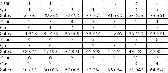
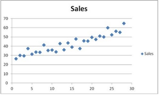 The scatterplot shows that the quarterly sales have an increasing trend and seasonality. A linear regression model given by Sales = β0 + β1Qtr1 + β2Qtr2 + β3Qtr3 + β4t + ε, where t is the time period (t = 1, ..., 28) and Qtr1, Qtr2, and Qtr3 are quarter dummies, is estimated and then used to make forecasts. For the regression model, the following partial output is available.
  Using MSE and MAD, compare the linear trend equation with seasonal dummy variables,
  t = 31,9261 - 7.855Qtr1 - 4.7362Qtr2 - 7.1656Qtr3 + 1.0749t, and the decomposition method equation
  t =
t =  t ×
t ×  t with
  t = 26.8819 + 1.0780t and the quarterly seasonal indices: 0.9322, 1.0066, 0.9441, and 1.1171. Which of the two corresponding forecasting models is recommended?
Correct Answer:
Verified
View Answer
Unlock this answer now
Get Access to more Verified Answers free of charge
Q115: The following table shows the annual revenues
Q116: Based on quarterly data collected over the
Q117: Which of the following components does not
Q118: If there are T observations to estimate
Q119: Quarterly sales of a department store for
Q120: Prices of crude oil have been steadily
Q121: Quarterly sales of a department store for
Q122: Quarterly sales of a department store for
Q123: Quarterly sales of a department store for
Q125: Quarterly sales of a department store for
Unlock this Answer For Free Now!
View this answer and more for free by performing one of the following actions

Scan the QR code to install the App and get 2 free unlocks

Unlock quizzes for free by uploading documents