The following table shows the annual revenues (in millions of dollars)of a pharmaceutical company over the period 1990-2011. 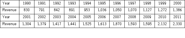 The autoregressive models of order 1 and 2,yt = β0 + β1yt - 1 + εt,and yt = β0 + β1yt - 1 + β2yt - 2 + εt,were applied on the time series to make revenue forecasts.The relevant parts of Excel regression outputs are given below.
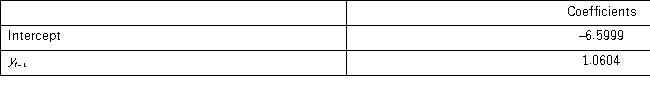
Model AR(1): 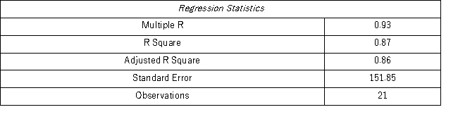
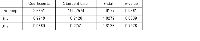
 Model AR(2):
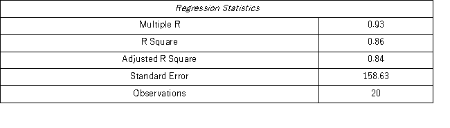
 When for AR(1),H0: β0 = 0 is tested against HA: β0 ≠ 0,the p-value of this t test shown by Excel output is 0.9590.This could suggest that the model yt = β1yt-1 + εt might be an alternative to the AR(1)model yt = β0 + β1yt-1 + εt.Excel partial output for this simplified model is as follows:
 (Use Regression in Data Analysis of Excel. )
Compare the autoregressive models yt = β0 + β1yt-1 + εt;yt = β0 + β1yt-1 + β2yt-2 + εt,andyt = β1yt-1 + εt,through the use of MSE and MAD.
Correct Answer:
Verified
View Answer
Unlock this answer now
Get Access to more Verified Answers free of charge
Q107: Prices of crude oil have been steadily
Q108: Quarterly sales of a department store for
Q109: Given the estimated model Q109: When using Excel for calculating moving averages, Q110: Prices of crude oil have been steadily Q111: The following table shows the annual revenues Q113: Prices of crude oil have been steadily Q115: The following table shows the annual revenues Q116: The model Q117: Which of the following components does not![]()
![]()
Unlock this Answer For Free Now!
View this answer and more for free by performing one of the following actions

Scan the QR code to install the App and get 2 free unlocks

Unlock quizzes for free by uploading documents